Visual Odometry Pipeline Explained
DEEP DIVE
When we talk about machines seeing, what we really mean is: can they understand how the world changes when they move?
Give a robot one eye. No GPS. No LiDAR. No depth sensor. Drop it into an unfamiliar space. Its only job? Figure out how it’s moving — just by noticing how the world around it shifts from frame to frame.
Or lets say you're standing in a dark room. No idea where you are. But you have a camera in your hand. You take a picture. Then you take a small step forward, and take another.
Now you look at the two images side by side and ask:
“What in this scene stayed the same… and what changed?”
“And based on that change, can I figure out how I moved?”
That’s the core idea behind Visual Odometry (VO).
It’s how we teach a camera to observe motion and infer structure — the same way we can close one eye and still walk through a room without bumping into a table.
Visual Odometry is the process of estimating a camera movement over time by analyzing how the scene appears to change in consecutive images.
It doesn’t try to recognize the world.
It doesn’t need to know what it’s looking at.
It just watches how things move.
If a chair appears slightly to the left in the second frame, and the wall has shifted downward, the camera infers:
“I must have moved slightly to the right and tilted upward.”
This is known as egomotion — the self-motion of the observer.
Let’s break down the Visual Odometry Pipeline.
Step 1: Find what stands out (Feature Detection)
We start by capturing two consecutive images from a moving camera. The goal is to identify features that remain consistent between these frames, despite the camera's movement. These consistent features, such as corners, blobs and edges, are known as keypoints - which are like little freckles in the image that stick out.
Feature Detection Algorithms:
SIFT (Scale-Invariant Feature Transform)
ORB (Oriented FAST and Rotated BRIEF)
FAST, AKAZE, and others - each with trade-offs
Each keypoint is also described — like giving it a fingerprint — using a vector of local pixel information (called a descriptor).
For ORB, these are binary.
For SIFT, they’re float vectors.
Either way, this is what makes matching possible.
Once we've found those visual anchors, the next question is - how do they move?
Read more about Feature Detectors here
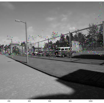
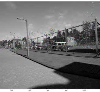
The colored circles are SIFT keypoints found for this image
Step 2: Find what's still there (Feature Matching)
Next, the camera looks at the next frame and asks:
“Do I still see that corner? That blob? That pattern?”
Matching descriptors between two images tells you what points correspond.
You can do this matching in different ways:
Brute-Force matcher — Compares every point with every other.
Fast for small data. Works well with ORB (using Hamming distance).FLANN matcher — Faster on larger datasets, especially with float descriptors like SIFT.
But matching is noisy. To filter bad matches, we apply Lowe’s Ratio Test:
“Is the best match significantly better than the second-best?
If not, don’t trust it.”
It keeps the ones you’re confident about — and throws the rest away.
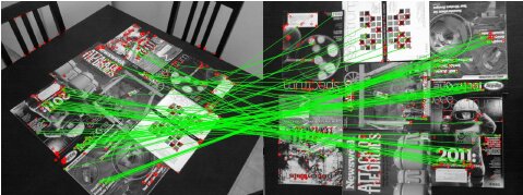
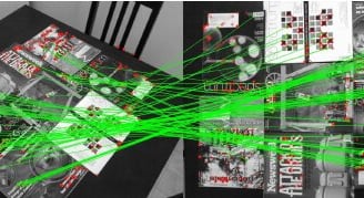
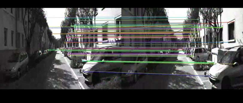
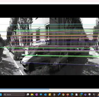
Image source: https://ieeexplore.ieee.org/document/6126544
Typical matching result using ORB on real-world images with viewpoint change. Green lines are valid matches; red circles indicate unmatched points.
Stripping Away the Camera's Influence
Before we get excited about geometry, we have to deal with one small problem:
The image coordinates we just matched aren’t “real.” They’re influenced by the quirks of the camera — its zoom level, the focal length, a shifted center point (where the image hits the sensor), slight stretching or skew from the lens.
So we clean them up.
We take those pixel coordinates and run them through the camera's intrinsic matrix — a 3×3 matrix that tells us how the camera projects the 3D world into 2D pixels - a fancy way of saying:
Before the camera can understand how it moved, it has to undo how the image was captured.
Every camera comes with its own intrinsics:
Focal length
Center offset (principal point)
Pixel scale and skew
These are encoded in a 3×3 matrix called the intrinsic matrix (K):
K = | fx 0 cx |
| 0 fy cy |
| 0 0 1 |
Where:
fx, fy are the focal lengths in pixels
cx, cy are the principal point offsets
When you match keypoints between two images, the points are still in pixel coordinates — influenced by all these internal parameters.
But here’s the problem:
Those pixel coordinates we’re working with? They’re distorted by these intrinsics.
And if you try to compute motion from them directly, your results will be warped — not by the world, but by the sensor.
So the first thing we do is ask the camera:
“Hey — forget your lens. Let’s just talk geometry.”
This means normalizing the keypoints:
Shifting them so the principal point is at the origin
Scaling them by the focal length
Turning pixel units into pure geometric rays
Once normalized, the points now live in a clean, camera-independent space. We’re ready to start asking deeper question
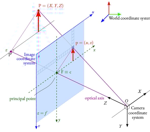
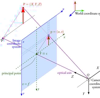
Pinhole camera model. Redrawn from OpenCV documentation
Image source: https://lhoangan.github.io/camera-params/
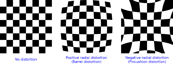
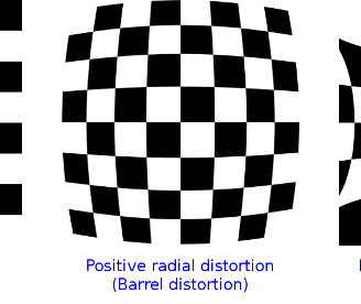
Example of radial distortions from imperfect lenses.
Step 3: Estimate Motion (Essential Matrix)
Once we have clean, matched keypoints in normalized coordinates, we can estimate how the camera moved between the two frames.
That motion is encoded in the Essential Matrix.
The Essential Matrix links the relative position and orientation of two cameras. When you decompose it, you get:
R – The rotation matrix (how the camera turned)
t – The translation vector (which direction it moved)
This is the core of motion estimation in monocular VO.
And since this is a single-camera setup, we only get the direction of motion — not the absolute scale.
The Essential Matrix is like a lens into the motion of the observer.
You feed it geometry, it tells you what movement could have caused it.
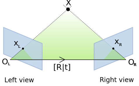
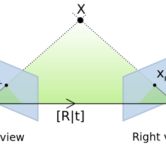
Image source: https://realitybytes.blog/tag/monocular-visual-odometry/
Graphic visualizing the Essential Matrix between two images.
Step 4: Chain the Motion (Pose Accumulation)
Each pair of frames gives us a relative pose — a little movement from the last step.
But to understand the full journey, we chain these poses together.
It’s like stacking transformation steps:
T_total = T1 @ T2 @ T3 @ ... @ Tn
Each pose is a 4×4 transformation matrix that combines rotation and translation (in SE(3)).
We track the camera’s global position over time by applying one movement after another. And just like that, you get a trajectory — a breadcrumb trail of where the camera has been.
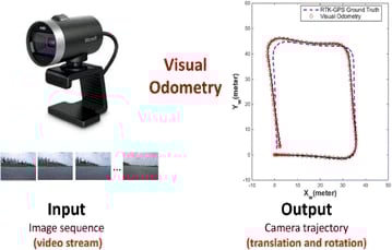
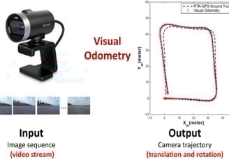
Camera Trajectory
Step 5: Rebuild the Scene (Triangulation)
Now comes the fun part.
Once you know where the camera was, and how the same point looked from two different views, you can figure out where that point lives in 3D space.
This is called triangulation.
Draw a ray from the camera’s position in Frame 1 toward the feature.
Draw another from Frame 2.
Where those two rays meet? That’s the point’s 3D position.
Do this for hundreds of points, and you get a sparse 3D map — a minimalist reconstruction of the environment.
It’s not pretty. But it’s functional.
We’re no longer just estimating motion — we’re giving the camera a memory of where things were.
Why Visual Odometry Still Matters
Visual Odometry is the first real-world perception tool most robots learn.
It powers:
SLAM (Simultaneous Localization and Mapping)
Indoor drone navigation
AR/VR headset tracking
Rovers on Mars
Self-driving car fallback systems
It works without GPS. Without LiDAR.
Just a camera and the willingness to watch how things change.
Resources:
1) Multiple view geometry in Computer Vision, Second edition. (n.d.). https://www.changjiangcai.com/files/text-books/Richard_Hartley_Andrew_Zisserman-Multiple_View_Geometry_in_Computer_Vision-EN.pdf